
What Is a Lorenz Curve?
 The Lorenz curve is a graphical representation showing the distribution of income or wealth within an economy developed by Max Lorenz in 1905.
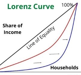
The Lorenz curve is a way to measure income distribution. The curve graphs cumulative percentages of income on the Y axis. It presents distribution as cumulative percentages of households on the X axis. If each group earns their share of the national income the Lorenz curve will be a straight line at a 45° angle. This is called the line of equality. For example, the bottom 10% earn 10% of national income, bottom 50% earn 50%, and so on.
An economy with an unequal distribution of income will create a Lorenz curve that is bowed out from the line of equality. For example, the bottom 25% earn 3% of national income, the bottom 50% earn 12%, and so on. Economies with a Lorenz curve farther from the line of equality have a less equal distribution of income. Conversely, economies with a Lorenz curve closer to the line of equality have a more equal distribution of income.
In practice, a Lorenz curve is usually a mathematical function estimated from an incomplete set of observations of income or wealth. It was developed by Max Lorenz in 1905 and is primarily used in economics. However, it may also be used to show inequality in other systems, for example, health care or access to education.
Reading a Lorenz Curve
The x-axis on a Lorenz curve typically shows distribution as represented by the percentage of the total population. The y-axis shows the share of total income or wealth. However, it can represent other values for whatever is being analyzed. Perfect equality would mean that a 1/x portion of the population controlled 1/x of the wealth. Therefore, perfect equality is represented as a straight line with a slope of 1. This line is often drawn on the graph as a means of reference. The curved line represents the actual wealth or income size distribution. The further away from the 1/1 baseline on a particular curve, the greater the inequality. Any point on the curve can be read to reveal what percentage or portion of the population control what percent of the wealth. Again, income is not the only variable that can be measured. Other systems can be studied as well.
Lorenz Curve – A Deeper Look
The Lorenz curve is often accompanied by a straight diagonal line with a slope of 1, which represents perfect equality in income or wealth distribution. The Lorenz curve is the curve beneath it. It graphically shows the observed or estimated distribution. The area between the straight line and the curved line, expressed as a ratio of the area under the straight line, is the Gini coefficient. It is a scalar measurement of inequality. The Lorenz curve is most often used to represent economic inequality.
However, it can also demonstrate unequal distribution in any system. The farther away the curve is from the straight diagonal line, the greater the degree of inequality. In economics, the Lorenz curve identifies inequality in the distribution of either wealth or income. However, these two are not identical or synonymous. It is possible to have high earnings but zero or negative net worth. Conversely, it is possible to have low earnings but large net worth.
A Lorenz curve usually starts with observable measurement of wealth or income distribution across a population. This measurement is based on data such as tax returns which report income for a large portion of the population. A graph of the data may be used directly as a Lorenz curve. Sometimes, economists and statisticians may fit a curve that represents a continuous function to fill in any gaps in the observed data. A Lorenz curve gives detailed information about the exact distribution of wealth or income across a population. It is more accurate than summary statistics like the Gini coefficient. Also, a Lorenz curve visually displays the distribution across each percentile or unit of measurement used to break down the data. Therefore, it can show precisely at which income or wealth percentiles the observed distribution varies from the line of equality.
Gini ratio vs Lorenz Curve
The Gini ratio is sometimes called the Gini coefficient or Gini Index. It is a numerical value derived from the Lorenz curve to measure income distribution. Using the areas from the Lorenz curve graph, the formula for the Gini ratio is:
Gini Ratio = A/(A+B)
The lower the Gini ratio is the more equal the country’s income distribution. A Country with a completely equal distribution of income, like pure socialism would have a coefficient closer to zero. Conversely, a country with a completely unequal distribution of income will have a Gini coefficient of 1. However, this could only occur if one person earns all of the income and everyone else owns nothing. Of course, neither extreme actually exists. But, in general, the higher the Gini coefficient, the more unequal the country’s distribution of income is. The CIA World Factbook has Gini ratios for many of the world’s economies.
Traditional Definition of the Gini Index
The Gini index or Gini coefficient is a statistical measure of distribution that was developed by the Italian statistician Corrado Gini in 1912. It is used as a gauge of economic inequality, measuring income distribution among a population. The coefficient ranges from 0 (or 0%) to 1 (or 100%), with 0 representing perfect equality and 1 representing perfect inequality. Values over 1 are not practically possible as we don’t take into account the negative incomes. Income can be 0 at its lowest but not negative.
For example, a country in which every resident has the same income would have an income Gini coefficient of 0. A country in which one resident earned all the income, while everyone else earned nothing, would have an income Gini coefficient of 1. The Gini coefficient is an important tool for analyzing income or wealth distribution within a country or region. But, Gini should not be mistaken as an absolute measurement of income or wealth.
What Shifts a Lorenz Curve?
Progressive income taxes shift the Lorenz curve inward toward the line of equality and lower the Gini ratio. Regressive Taxes are taxes where tax rates are higher for those earning less. Regressive taxes shift the Lorenz curve outward away from the line of equality and increase the Gini ratio.
How taxes and transfer payments change the Lorenz Curve and Gini ratio
Progressive Taxes are taxes where marginal tax rates increase as a person makes more income. A progressive tax system may charge a citizen 10% on the first $10,000 of income, 20% on next $30,000 ($10,001 – $40,000) and 30% on marginal income above $40,000. For example, a person earning $5,000 a year would pay $500 in taxes. A person earning $100,000 a year would pay $25,000 in taxes. Progressive income taxes shift the Lorenz curve inward toward the line of equality and lower the Gini ratio.
Regressive Taxes are taxes where tax rates are higher for those earning less. If a person earning $10,000 pays 10% of their income ($1000) to the regressive tax, a person earning $1,000,000 might pay %5 of their income ($50,000). The higher income earner might pay a higher amount in absolute terms. However, the person with less income pays a higher percentage. For example, sales taxes are considered a regressive tax. This is because low-income earners pay higher percentages of their income than high-income earners. Regressive taxes shift the Lorenz curve outward away from the line of equality and increase the Gini ratio.
Proportional Taxes are taxes where the marginal tax rate does not change based on income earned. If someone earning $10,000 pays 10% of their income, then someone earning $1,000,000 would also pay 10% of their income. Proportional taxes do not change the Lorenz curve or Gini ratio.
Transfer Payments are social programs for people with low income that provide subsidies or direct aid. Social security payments, unemployment compensation, food stamp programs, etc. are all examples of transfer payments. Transfer payments reduce income inequality and shift the Lorenz curve inward toward the line of equality. As a result, they reduce the Gini ratio.
Final Words
Constructing a Lorenz curve involves fitting a continuous function to an incomplete set of data. Therefore, there is no guarantee that the values along a Lorenz curve actually correspond to the true distributions of income. Except for those points that are actually observed data, most of the points along the curve are just guesses. But, those estimates are usually based on the shape of the curve that best fits the observed data points. Ultimately, the shape of the Lorenz curve can be influenced by the quality and sample size of the data. Also, by the mathematical assumptions and judgments as to what constitutes the best fit curve. As a result, these factors may represent sources of substantial error between the Lorenz curve and the actual distribution.
A high-income country and a low-income one can have the same Gini coefficient. This can happen when total income is different, but the incomes are distributed similarly within each country. One of the common market failures of modern capitalist economies is highly unequal distributions of income and wealth. Some economists argue extremely unequal distributions of income or wealth can lead to political instability and slow economic growth. Resources that would otherwise be used to create wealth are instead used to protect wealth.
Up Next: What Is a Posterior Probability?
 The posterior probability is the probability an event will happen after all evidence or background information has been taken into account. It is a revised probability that takes into account new available information.
In Bayesian statistics, it is the revised or updated probability of an event. However, the revision occurs after taking into consideration the existing as well as the new information. Specifically, it is the conditional probability of a given event. It is calculated after observing a second event whose conditional and unconditional probabilities were known in advance. It is computed by revising the prior probability. That is the probability assigned to the first event before observing the second event using Bayes’ theorem. In statistical terms, it becomes the probability of event A occurring given that event B has occurred.